Roll Diffusion Calculator
Quick Start
This calculates the diffusion of heat or humidity into a roll over time. It allows multiple options covering different diffusion scenarios.
Credits
This is taken from the old AbbottApps which are based on inputs from web-handling experts Dr David Roisum, Dr Dilwyn Jones and Tim Walker.
Roll Diffusion Calculator
//One universal basic required here to get things going once loaded
let DoTheCalc=false
window.onload = function () {
    //restoreDefaultValues(); //Un-comment this if you want to start with defaults
    Main();
};
// document.getElementById("Calc").addEventListener('click', DoIt, false);
// function DoIt(){
//     DoTheCalc=true
//     Main()
// }
//Main() is hard wired as THE place to start calculating when inputs change
//It does no calculations itself, it merely sets them up, sends off variables, gets results and, if necessary, plots them.
function Main() {
    //Save settings every time you calculate, so they're always ready on a reload
    saveSettings();

    //Send all the inputs as a structured object
    //If you need to convert to, say, SI units, do it here!
    const inputs = {
        D:sliders.SlideD.value,
        Width:sliders.SlideW.value,
        OD:sliders.SlideOD.value,
        RD:sliders.SlideRD.value,
        From:sliders.SlideFrom.value,
        To: sliders.SlideTo.value,
        Time: sliders.SlideTime.value,
        Open: document.getElementById('Open').checked,
        Sealed: document.getElementById('Sealed').checked,
        Fixed: document.getElementById('Fixed').checked,
        Full: document.getElementById('Full').checked,
    };


    //Send inputs off to CalcIt where the names are instantly available
    //Get all the resonses as an object, result
    const result = CalcIt(inputs);
    if (result.plots) {
        for (let i = 0; i < result.plots.length; i++) {
            plotIt(result.plots[i], result.canvas[i]);
        }
    }

    //You might have some other stuff to do here, but for most apps that's it for Main!
}

//Here's the app calculation
//The inputs are just the names provided - their order in the curly brackets is unimportant!
//By convention the input values are provided with the correct units within Main
function CalcIt({D,Width,OD, RD, From, To, Time, Open, Sealed, Fixed, Full }) {
     const theCanvas =document.getElementById('canvas');
    ctx = theCanvas.getContext("2d");
    cw=theCanvas.width;ch=theCanvas.height
    ctx.fillStyle="blue"
    ctx.rect(0,0,cw,ch)
    ctx.fill()
    // if (!DoTheCalc){
    //     return {
    //         plots: [prmap],
    //         canvas: ['canvas1'],
    //     };

    // }

    DoTheCalc=false
    let MinP=From
    let MaxP=To
    if (MaxP1000) {RSteps*=1/(1+(Time-1000)/8000)}
              RSteps=Math.floor(RSteps)
              if (RSteps/2-Math.floor(RSteps/2)>0.01) RSteps-=1
              Time*=3600 //Hrs to secs
              const FromVal = From;
              const ToVal = To;
              if (ToVal==FromVal) {ToVal=FromVal+10}

			//Set up the graphics

			const RadOut = RDiameter/ 2000
			const RadIn = RCore / 2000
			const TheLength = WebWidth
			const ZSteps = Math.floor(RSteps * TheLength / (RadOut - RadIn)/2)

			let R2 = Math.floor(RSteps/2) , Z2 = Math.floor(ZSteps/2)
			const Beta = DiffCoef/1e4 //cm2 to m2
			VFrom = FromVal
			VTo = ToVal
			const TMax = Time //Seconds
			const Volume = Math.PI * (RadOut*RadOut -RadIn*RadIn) * TheLength
			const DR = (RadOut - RadIn) / RSteps
			const CoreIsolated = Sealed
			const CoreFixed = Fixed

			if (CoreIsolated)  R2 = 1
			const DZ = TheLength / ZSteps
			const DR2 = DR*DR ,DZ2 = DZ*DZ
			const DT = 1 / Beta / (1 / DR2 + 1 / DZ2) / 4
			const TimPts = Math.max(1, TMax / DT)
			//console.log (RSteps,ZSteps,DT,TMax, Beta, DR2,DZ2)
			if (TimPts > 100000)
			{
				alert("This is likely to be too slow! Reduce your TMax or increase your roll diameter")
				return
			}
			const BetaDT = Beta * DT
			const Term3 = BetaDT / DZ2
			const Term4 = BetaDT / DZ2
			const Term5 = (1 - (1 / DR2 + 1 / DZ2) * 2 * BetaDT)
			//Set everything to initial value
			const C0 =[],C1=[],RFact=[]
			let tmp=[]
			let R,Z
			for (R = 0 ;R<= RSteps; R++)
			{
			tmp=RadIn+R/RSteps*(RadOut-RadIn)
			RFact[R]=tmp*tmp/(RadIn*RadIn)
				C0[R]=[];C1[R]=[]
				for (Z = 0 ; Z<=ZSteps; Z++)
				{
					C0[R][Z] = VFrom;C1[R][Z] = VFrom
				}
			}
			//Set boundaries
			for( R = 0; R<=RSteps; R++)
			{
				C0[R][0] = VTo
				C0[R][ZSteps] = VTo
			}
			for (Z = 0 ; Z<= ZSteps; Z++)
			{
				if (!CoreIsolated && (!CoreFixed )) C0[0][Z] = VTo
				C0[RSteps][Z] = VTo
			}
			let Diff = 0
			let DiffW=0
			for (R = 1;R< RSteps;R++)
			{
				for (Z = 1 ;Z< ZSteps; Z++)
				{
					Diff += Math.abs(VTo - C0[R][Z])
					DiffW+=Math.abs(VTo - C0[R][Z])*RFact[R]
				}
			}

			const DiffMax = Diff
			const DiffMaxW=DiffW
			const PPts =[], PPts2=[],PPtsW=[]
			PPts.push({x:0,y:VFrom});PPts2.push({x:0,y:VFrom});PPtsW.push({x:0,y:VFrom})
			//The big loop
			let NextTim=0, TimStep= Math.floor(TimPts / 100)
			let x, y
			const RadR=[]
			for (R=0;R<=RSteps;R++)
			{RadR[R]=RadIn+R*DR}
			for (Tim = 1 ;Tim<= TimPts;Tim++)
			{
				for (R = 1; R< RSteps;R++)
				{
					Rad = RadR[R]
					for (Z = 1;Z= NextTim)
				{
					x = Tim*DT/3600
					y =  (1 - Diff / DiffMax)
					y=VFrom+y*(VTo-VFrom)
					PPts.push({x:x,y:y})
					y =  (1 - DiffW / DiffMaxW)
					y=VFrom+y*(VTo-VFrom)
					PPtsW.push({x:x,y:y})
					y = (Math.abs((C0[R2][Z2] - VFrom) / (VTo - VFrom)))
					y=VFrom+y*(VTo-VFrom)
					PPts2.push({x:x,y:y})
					NextTim += TimStep
				}
			}
            const yheight=200
			const blocx=Math.floor(290/ZSteps)
			const blocy=Math.floor(yheight/RSteps)
			const AmFull= Full
			const FullDiv=2.05+RadIn/RadOut
            ctx.clearRect(0,0,cw,ch)
            let rbow
			for (R = 0;R<= RSteps;R++)
			{
				for (Z = 0 ;Z<= ZSteps; Z++)
				{
					rbow = Rainbow(Math.abs((VTo - C0[R][Z]) / (VTo - VFrom)))
                    ctx.fillStyle="rgb(" + rbow.r + "," + rbow.g + "," + rbow.b + ")"
                    if (AmFull)
					{
                        ctx.fillRect(Z*blocx,(RSteps-R)*blocy/FullDiv,blocx,blocy/2)
                        ctx.fillRect(Z*blocx,yheight-(RSteps-R)*blocy/FullDiv,blocx,blocy/2)
					}
					else
					{
                        ctx.fillRect(Z*blocx,(RSteps-R)*blocy,blocx,blocy)
				}
				}
			}
			let CoreText="Core Open"
			if (CoreIsolated) {CoreText="Core Sealed"}
			if (CoreFixed) {CoreText="Core Fixed"}
			if (AmFull) CoreText=""
            ctx.font = "12pt Verdana, sans-serif";
            ctx.fillStyle="white"
            ctx.fillText(CoreText,blocx*ZSteps/3,180);
            const plotData = [PPts,PPtsW,PPts2]
            const lineLabels = ["LinAv","VolAv","Furthest"]
            const prmap = {
                plotData: plotData, //An array of 1 or more datasets
                lineLabels: lineLabels, //An array of labels for each dataset
                hideLegend: false, //Set to true if you don't want to see any labels/legnds.
                xLabel: 't&hrs', //Label for the x axis, with an & to separate the units
                yLabel: 'Value& ', //Label for the y axis, with an & to separate the units
                y2Label: null, //Label for the y2 axis, null if not needed
                yAxisL1R2: [], //Array to say which axis each dataset goes on. Blank=Left=1
                logX: false, //Is the x-axis in log form?
                xTicks: undefined, //We can define a tick function if we're being fancy
                logY: false, //Is the y-axis in log form?
                yTicks: undefined, //We can define a tick function if we're being fancy
                legendPosition: 'top', //Where we want the legend - top, bottom, left, right
                xMinMax: [0,], //Set min and max, e.g. [-10,100], leave one or both blank for auto
                yMinMax: [Math.min(From,To),Math.max(From,To)], //Set min and max, e.g. [-10,100], leave one or both blank for auto
                y2MinMax: [,], //Set min and max, e.g. [-10,100], leave one or both blank for auto
                xSigFigs: 'F2', //These are the sig figs for the Tooltip readout. A wide choice!
                ySigFigs: 'F2', //F for Fixed, P for Precision, E for exponential
            };


    //Now we return everything - text boxes, plot and the name of the canvas, which is 'canvas' for a single plot
    return {
        plots: [prmap],
        canvas: ['canvas1'],


    };
}

let RB = [[0, 48, 245], [0, 52, 242], [0, 55, 238], [0, 59, 235], [3, 62, 231], [9, 66, 228], [14, 69, 225], [18, 72, 221], [20, 74, 218], [22, 77, 214], [23, 80, 211], [24, 82, 207], [25, 85, 204], [25, 87, 200], [25, 90, 197], [25, 92, 193], [25, 94, 190], [25, 96, 187], [24, 99, 183], [24, 101, 180], [24, 103, 177], [23, 105, 173], [23, 106, 170], [24, 108, 167], [24, 110, 164], [25, 112, 160], [27, 113, 157], [28, 115, 154], [30, 117, 151], [32, 118, 148], [34, 120, 145], [36, 121, 142], [39, 122, 139], [41, 124, 136], [43, 125, 133], [45, 126, 130], [47, 128, 127], [49, 129, 124], [51, 130, 121], [53, 132, 118], [54, 133, 115], [56, 134, 112], [57, 136, 109], [58, 137, 106], [59, 138, 103], [60, 139, 99], [61, 141, 96], [62, 142, 93], [62, 143, 90], [63, 145, 87], [63, 146, 83], [64, 147, 80], [64, 149, 77], [64, 150, 74], [65, 151, 70], [65, 153, 67], [65, 154, 63], [65, 155, 60], [66, 156, 56], [66, 158, 53], [67, 159, 50], [68, 160, 46], [69, 161, 43], [70, 162, 40], [71, 163, 37], [73, 164, 34], [75, 165, 31], [77, 166, 28], [79, 167, 26], [82, 168, 24], [84, 169, 22], [87, 170, 20], [90, 171, 19], [93, 172, 18], [96, 173, 17], [99, 173, 17], [102, 174, 16], [105, 175, 16], [108, 176, 16], [111, 176, 16], [114, 177, 17], [117, 178, 17], [121, 179, 17], [124, 179, 18], [127, 180, 18], [130, 181, 19], [132, 182, 19], [135, 182, 20], [138, 183, 20], [141, 184, 20], [144, 184, 21], [147, 185, 21], [150, 186, 22], [153, 186, 22], [155, 187, 23], [158, 188, 23], [161, 188, 24], [164, 189, 24], [166, 190, 25], [169, 190, 25], [172, 191, 25], [175, 192, 26], [177, 192, 26], [180, 193, 27], [183, 194, 27], [186, 194, 28], [188, 195, 28], [191, 195, 29], [194, 196, 29], [196, 197, 30], [199, 197, 30], [202, 198, 30], [204, 199, 31], [207, 199, 31], [210, 200, 32], [212, 200, 32], [215, 201, 33], [217, 201, 33], [220, 202, 34], [223, 202, 34], [225, 202, 34], [227, 203, 35], [230, 203, 35], [232, 203, 35], [234, 203, 36], [236, 203, 36], [238, 203, 36], [240, 203, 36], [241, 202, 36], [243, 202, 36], [244, 201, 36], [245, 200, 36], [246, 200, 36], [247, 199, 36], [248, 197, 36], [248, 196, 36], [249, 195, 36], [249, 194, 35], [249, 192, 35], [250, 191, 35], [250, 190, 35], [250, 188, 34], [250, 187, 34], [250, 185, 34], [250, 184, 33], [250, 182, 33], [250, 180, 33], [250, 179, 32], [249, 177, 32], [249, 176, 32], [249, 174, 31], [249, 173, 31], [249, 171, 31], [249, 169, 30], [249, 168, 30], [249, 166, 30], [248, 165, 29], [248, 163, 29], [248, 161, 29], [248, 160, 29], [248, 158, 28], [248, 157, 28], [248, 155, 28], [247, 153, 27], [247, 152, 27], [247, 150, 27], [247, 148, 26], [247, 147, 26], [246, 145, 26], [246, 143, 26], [246, 142, 25], [246, 140, 25], [246, 138, 25], [245, 137, 24], [245, 135, 24], [245, 133, 24], [245, 132, 24], [244, 130, 23], [244, 128, 23], [244, 127, 23], [244, 125, 23], [244, 123, 22], [243, 121, 22], [243, 119, 22], [243, 118, 22], [243, 116, 21], [242, 114, 21], [242, 112, 21], [242, 110, 21], [241, 109, 21], [241, 107, 21], [241, 105, 21], [241, 103, 21], [240, 101, 21], [240, 100, 22], [240, 98, 22], [240, 96, 23], [240, 95, 24], [240, 93, 26], [240, 92, 27], [240, 90, 29], [240, 89, 31], [240, 88, 33], [240, 87, 36], [240, 87, 38], [241, 86, 41], [241, 86, 44], [242, 86, 47], [242, 86, 51], [243, 86, 54], [243, 87, 58], [244, 88, 62], [245, 88, 65], [245, 89, 69], [246, 90, 73], [247, 91, 77], [247, 92, 82], [248, 94, 86], [249, 95, 90], [249, 96, 94], [250, 97, 98], [251, 99, 102], [251, 100, 106], [252, 101, 111], [252, 103, 115], [253, 104, 119], [253, 105, 123], [254, 107, 128], [254, 108, 132], [255, 109, 136], [255, 111, 140], [255, 112, 145], [255, 114, 149], [255, 115, 153], [255, 116, 157], [255, 118, 162], [255, 119, 166], [255, 120, 170], [255, 122, 175], [255, 123, 179], [255, 125, 183], [255, 126, 188], [255, 127, 192], [255, 129, 196], [255, 130, 201], [255, 132, 205], [255, 133, 210], [255, 134, 214], [255, 136, 219], [255, 137, 223], [255, 139, 227], [255, 140, 232], [255, 141, 236], [254, 143, 241], [254, 144, 245], [253, 146, 250]]
function Rainbow(v) {
    var i = Math.floor((Math.min(v, 1), Math.max(v, 0)) * 255)
    r = RB[i][0]
    g = RB[i][1]
    b = RB[i][2]
    return { r: r, g: g, b: b }
}
Diffusion Calculations
Once your roll is wound, you might be interested to know how its temperature might change if placed into a hot or cold store, or how humidity might vary throughout the roll or how solvent vapours will diffuse out of the roll.
The calculations for all three cases are the same. They all require the obvious basics: Roll diameter, Core diameter and Roll width. They need a From value (e.g 30 for 30deg or 30%RH) and a To value (e.g. 5 for 5deg or 5%RH). And they need an estimate, Time, in hours of the timescale for diffusion. If you select too short a Time then you will get a curve that hardly changes across the width. If it’s too large then your first data point will reach equilibrium. Long timespans take a long time to calculate, so always use smaller Times when you are first experimenting.
Finally, the calculations need a Diffusivity. Note that the model assumes linear, isotropic properties – so the diffusion coefficient is the same in the axial and radial directions, and diffusion obeys Fick’s Laws.
Not many of us know values of diffusivities. A typical value for a polyester web and question of thermal equilibration is 0.001cm²/s. A typical value for a paper roll and hygroscopic equilibration is 0.0001. But in real life you will have to do some measurements on a small roll (which equilibrates quickly, making it easy to do the experiments) by which you calibrate the diffusivity value that you can use on larger rolls (where experimentation is much more difficult).
To experimentally determine the effective thermal diffusivity you can bury a thermocouple in a wound roll. Change the Diffusivity value in the RDC until the temperature predicted matches the temperature measured at that location. To be most practical, the thermocouple should be as far from all edges as practical and the roll chosen to be of a size that could cool noticeably in a few hours or a few days.
To experimentally determine the effective hygroscopic diffusivity you merely need to weigh, over time, a small (drying/wetting) roll and change Diffusivity value in the RDC until calculations match measurements. To be most practical, you should trial something like a delta of 5% moisture (such as 10% > 5%) in about the range you will be most interested in (because hygroscopic diffusivity is not truly a constant like it is with thermal problems). Also, roll size should be small enough to noticeably change weight in a few days. This would be something about the size of a loaf of bread which could be obtained as a butt roll from your slitter rewinders.
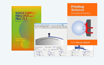
On pressing Calculate you see two things.
- The graph has two lower lines representing the volumetric and linear average deviation of the roll from equilibrium which show a typical exponential shape. The volumetric line decreases faster because the bulk of the roll is on the outside (larger radius). If you change values of From and To you may be surprised to see that the curves do not change! And it has no idea if it is calculating temperatures, humidities or solvents. The shape is characteristic only of the size of the roll and the diffusivity. If you move the mouse over the graph you get a readout of the values at different times. The graph also shows a line (top) showing the value at the part of the roll which is furthest from the outside and therefore the slowest to respond. The curves give you complementary information – some users are more interested in one value than the other.
- A rainbow-coloured map showing deviations from equilibrium across the roll which you see in semi cross-section (i.e. the other half of the roll is not shown because it is identical to the top half). The core is at the bottom of the image, along with text reminding you of the setup. Red is the furthest from equilibrium, blue is equilibrium. As time goes on, the map gets closer to the uniform blue colour. If Full mode is chosen then the roll is shown in full with a core (not to scale!) in the middle. This mode reduces resolution but gives a clearer picture of what is happening.
There is one more choice to make. The calculations assume that the outer and inner layers of the roll are in complete equilibrium (thermal, hygroscopic etc.) with the surrounding air. This may or may not be realistic, but it’s a reasonable assumption for many cases. However, if you are using an impermeable core (e.g. plastic) then no humidity (or solvent) can diffuse in or out of the core. In this case, select the Core Sealed option. Now diffusion will be much slower as one diffusion pathway is blocked. And if for some reason the core is held at the fixed “From” temperature, then selecting the Core Fixed option means that each part of the roll will reach an equilibrium value balanced between the outside and the inside conditions.