
Controlled Release (Higuchi)
Quick Start
It is common to add solute particles to a polymer providing controlled release into the environment for medical or agricultural uses. This can be modelled via Higuchi kinetics. Here we use a rectangular geometry and assume that the Higuchi assumptions are valid.
Comments
There are variants (cylinders, rings, boundaries, swelling) that can be incorporated if users want them.
Controlled Release (Higuchi)
"use strict"
const dtos = 3600 * 24
//One universal basic required here to get things going once loaded
window.onload = function () {
    //restoreDefaultValues(); //Un-comment this if you want to start with defaults
    Main();
};

//Main() is hard wired as THE place to start calculating when inputs change
//It does no calculations itself, it merely sets them up, sends off variables, gets results and, if necessary, plots them.
function Main() {
    //Save settings every time you calculate, so they're always ready on a reload
    saveSettings();

    //Send all the inputs as a structured object
    //If you need to convert to, say, SI units, do it here!
    const inputs = {
        D: parseFloat(document.getElementById('D').value),
        hp: sliders.Slidehp.value / 10, //mm to cm
        tmax: sliders.Slidetmax.value * dtos, //d to s
        Cp: sliders.SlideCp.value,
        Cs: sliders.SlideCs.value,
        A: sliders.SlideA.value,
    };

    //Send inputs off to CalcIt where the names are instantly available
    //Get all the resonses as an object, result
    const result = CalcIt(inputs);

    //Set all the text box outputs
    document.getElementById('initial').value = result.initial;
    document.getElementById('remaining').value = result.remaining;
    document.getElementById('released').value = result.released;
    document.getElementById('releasedperc').value = result.releasedperc;
    document.getElementById('hend').value = result.hend;
    document.getElementById('tend').value = result.tend;
    //Do all relevant plots by calling plotIt - if there's no plot, nothing happens
    //plotIt is part of the app infrastructure in app.new.js
    if (result.plots) {
        for (let i = 0; i < result.plots.length; i++) {
            plotIt(result.plots[i], result.canvas[i]);
        }
    }
    //You might have some other stuff to do here, but for most apps that's it for Main!
}

//Here's the app calculation
function CalcIt({ D, Cp, Cs, hp, A, tmax }) {
    let m, h, Plotm = [], Blank = [], nextt = 0, t = 0
    if (Cp > 5 * Cs) {

        for (t = 0; t <= tmax; t++) {
            m = A * Math.sqrt((2 * Cp - Cs) * D * t * Cs)
            h = 2 * Math.sqrt((D * t * Cs) / (2 * Cp - Cs))
            if (h > hp * 1.01) { //Looks a bit nicer
                m = A * hp * Cp; h = hp
                Plotm.push({ x: t / dtos, y: 100 * m / (A * hp * Cp) })
                break
            }
            if (t >= nextt) {
                Plotm.push({ x: t / dtos, y: 100 * m / (A * hp * Cp) })
                nextt += tmax / 200
            }
        }
    }
    const tend = t / dtos
    const initial = A * hp * Cp
    const released = m
    const releasedperc = 100 * m / (A * hp * Cp)
    const remaining = 100 * (1 - m / (A * hp * Cp))
    const hend = h * 10

    const plotData = Cp > 5 * Cs ? [Plotm] : [Blank], lineLabels = ["m"], myColors = ["blue"], borderWidth = [3]

    //Now set up all the graphing data detail by detail.
    const prmap = {
        plotData: plotData, //An array of 1 or more datasets
        lineLabels: lineLabels, //An array of labels for each dataset
        colors: myColors, //An array of colors for each dataset
        hideLegend: true,
        borderWidth: borderWidth,
        xLabel: 't&d', //Label for the x axis, with an & to separate the units
        yLabel: 'Released&%', //Label for the y axis, with an & to separate the units
        y2Label: null, //Label for the y2 axis, null if not needed
        yAxisL1R2: [], //Array to say which axis each dataset goes on. Blank=Left=1
        logX: false, //Is the x-axis in log form?
        xTicks: undefined, //We can define a tick function if we're being fancy
        logY: false, //Is the y-axis in log form?
        yTicks: undefined, //We can define a tick function if we're being fancy
        legendPosition: 'top', //Where we want the legend - top, bottom, left, right
        xMinMax: [,], //Set min and max, e.g. [-10,100], leave one or both blank for auto
        yMinMax: [0,], //Set min and max, e.g. [-10,100], leave one or both blank for auto
        y2MinMax: [,], //Set min and max, e.g. [-10,100], leave one or both blank for auto
        xSigFigs: 'F1', //These are the sig figs for the Tooltip readout. A wide choice!
        ySigFigs: 'F3', //F for Fixed, P for Precision, E for exponential
    };

    //Now we return everything - text boxes, plot and the name of the canvas, which is 'canvas' for a single plot
    if (Cp < 5 * Cs) {
        return {
            plots: [prmap],
            canvas: ['canvas'],
            initial: "n/a",
            released: "n/a",
            releasedperc: "n/a",
            remaining: "n/a",
            hend: "n/a",
            tend: "n/a",
        };
    } else {
        return {
            plots: [prmap],
            canvas: ['canvas'],
            initial: initial.toPrecision(3),
            released: released.toPrecision(3),
            releasedperc: releasedperc.toFixed(1),
            remaining: remaining.toFixed(1),
            hend: hend.toFixed(2),
            tend: tend.toFixed(2),
        };
    }
}
 Controlled release
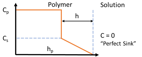
There are many variants but here we take the standard scenario. Small particles of a solute are added to a polymer (or gel or cream or elastomer ... we'll call them all "polymer") at a concentration Cp way above the solubility of the solute in the polymer, Cs. The polymer (assumed to be a rectangle) has an area A in contact with the solvent and a thickness hp. If both surfaces of the polymer are in contact with the solvent then the hp is half the real thickness.
The solute saturates the polymer and diffuses out with diffusion coefficient D. As it exits, solute transfers from the particles to keep the concentration at Cs. As the process continues (with "perfect sink" conditions assumed so C = 0 in the solution), a front moves a distance h into the polymer. The inner part is at average concentration Cp and the outer part is a linear gradient from Cs down to 0. The simulation time is tmax in days, but stops automatically if 100% of the solute has been released.
The Higuchi equation
The mass M released from the polymer at time t is given by the Higuchi equation:
`M=A\sqrt((2C_p-C_s)DtC_s)`
The distance, h, of the front from the solvent interface is given by:
`h=2\sqrt((DtC_s)/((2C_p-C_s)))`
The standard equation has no way to produce a graceful end to the diffusion once h = hp. Initial versions of the app just stopped at this point, but it seemed better to add an artificial smooth transition to 100%.
Units
The concentrations are %wt/vol, assumed to be %g/cc. The internal calculations are all in cm (D values are cm²/s, usually typed as "exponential format" e.g. 3.2e-9) so the total weight of solute is just CphpA. This allows us to calculate absolute and relative concentrations released. The position of the front at the end of your chosen time tmax is also recorded, in mm, though this will be hp if the front has reached the limit.
Higuchi Assumptions
The standard assumptions turn out to be pretty reliable across many real-world systems:
- Diffusion is effectively 1D from a planar sample
- The particles are small (relative to the sample thickness) and evenly distributed
- Diffusion through the polymer is the limiting factor
- Diffusion into the solvent is fast
- The particle dissolution to re-saturate the polymer is also fast
- The diffusion coefficient is constant
- No concentration-dependent diffusion
- No swelling of the polymer to increase D
- We have "perfect sink" conditions so the external concentration is always zero
- Cp >> Cs (the app will show "n/a" if the ratio is less than 5)
- There is no swelling or erosion of the polymer - i.e. its dimensions are stable
If you want options for spherical, cylindrical or toroidal geometries, or want to include other effects, let me know and I'll try to add them.
For solutes that are dissolved in the polymer, the standard Fickian Diffusion app should be used.