Young-Laplace
Quick Start
You have a drop of fluid A in fluid B. Thanks to a difference in densities, the drop will deform under gravity, resisted by the intefacial tension. The Young-Laplace equation describes that balance. From an image of the drop and a bit of fitting, you can work out the IFT.
Credits
The Osaka U team led by Masashi Nakamoto provided the core papers1,2 that inspired the app.
Young-Laplace
'use strict'
//One universal basic required here to get things going once loaded
let image,edge,edgemin,edgemax, imgWidth, imgHeight, context, imageData,oldImageData, oldAngle = 0, xMin,xMax,yMin,yMax

window.onload = function () {
    //restoreDefaultValues(); //Un-comment this if you want to start with defaults
    document.getElementById('Load').addEventListener('click', clearOldName, false);
    document.getElementById('Load').addEventListener('change', handleFileSelect, false);

    loadAndDrawImage("img/Test.png")
    //loadAndDrawImage("img/TestDrop.jpg")
    Main();
};
//Any global variables go here


//Main is hard wired as THE place to start calculating when input changes
//It does no calculations itself, it merely sets them up, sends off variables, gets results and, if necessary, plots them.
function Main() {
    saveSettings();

    //Send all the inputs as a structured object
    //If you need to convert to, say, SI units, do it here!
    const inputs = {
        h: sliders.Slideh.value / 1e3,
        b: sliders.Slideb.value / 1e3,
        delta: sliders.Slidedelta.value * 1e3,
        sigma: sliders.Slidesigma.value / 1e3,
        mm: sliders.Slidemm.value,
        Base: sliders.SlideBase.value,
        Xoffs: sliders.SlideXoffs.value,
        Xrange: sliders.SlideXrange.value,
        Yrange: sliders.SlideYrange.value,
       Angle: sliders.SlideAngle.value * Math.PI / 180, //Deg to Rad
    }
    //These are convenient as direct global variables
        xMin = sliders.SlidexMin.value/100 //From %
        xMax = sliders.SlidexMax.value/100 //From %
        yMin = sliders.SlideyMin.value/100 //From %
        yMax = sliders.SlideyMax.value/100 //From %

    //Send inputs off to CalcIt where the names are instantly available
    //Get all the resonses as an object, result
    const result = CalcIt(inputs)

    //Set all the text box outputs
    document.getElementById('Volume').value = result.Volume
    document.getElementById('Width').value = result.Width

    //Do all relevant plots by calling plotIt - if there's no plot, nothing happens
    //plotIt is part of the app infrastructure in app.new.js
    if (result.plots) {
        for (let i = 0; i < result.plots.length; i++) {
            plotIt(result.plots[i], result.canvas[i]);
        }
    }

    //You might have some other stuff to do here, but for most apps that's it for CalcIt!
}

//Here's the app calculation
//The inputs are just the names provided - their order in the curly brackets is unimportant!
//By convention the input values are provided with the correct units within Main
function CalcIt({  h, b, delta, sigma, mm, Base, Xoffs, Xrange, Yrange, Angle }) {
    if (oldImageData!=null) DoStuff(Base, mm, Angle)
    let tmp = [], DPlot = [],EPlot=[], z = h, x = 0, phi = 0, Volume = 0,  R = 2 * b, dz = 0
    const phiinc = 0.001,pi = Math.PI, g = 9.81, dgs = delta * g / sigma
    let maxWidth = 0
    for (phi = 0; phi < pi; phi += phiinc) {
        tmp.push({ x: x * 1e3, y: -z * 1e3 })
        x += R * Math.cos(phi) * phiinc
        maxWidth = Math.max(x, maxWidth)
        dz = R * Math.sin(phi) * phiinc
        z -= dz
        R = 1 / (dgs * (h - z) + 2 / b - Math.sin(phi) / x)
        Volume += pi * dz * x * x
        if (z < 0) break
    }
    const tl = tmp.length - 1
    for (let i = 0; i <= tl; i++) {
        DPlot.push({ x: -tmp[tl - i].x, y: tmp[tl - i].y })
    }
    for (let i = 0; i < tmp.length; i++) {
        DPlot.push({ x: tmp[i].x, y: tmp[i].y })
    }
    //Now plot the edge, suitable scales/centered
    if (edge){
        const mmW=mm/imgWidth
        const correction=mm/2+(edgemin*mmW-edgemax*mmW)/2
    // for (let i=0; i imgWidth*xMin && edge[i].x < imgWidth*xMax && edge[i].y > imgHeight*yMin && edge[i].y < imgHeight*yMax)  EPlot.push({ x: edge[i].x * mmW - correction + Xoffs, y: Base + ( - edge[i].y) * mmW })
        }
   }
    //Now set up all the graphing data detail by detail.
    let plotData = [DPlot,EPlot]
    let lineLabels = ["Calculated","Edge"] //An array of labels for each dataset
    let xMM=[],yMM=[]
    if (document.getElementById("Magnify").checked){
        xMM.push(-Xrange);xMM.push(Xrange)
        yMM.push(-h*1e3);yMM.push(-h*1e3+Yrange)
    } else {
        xMM.push();xMM.push()
        yMM.push();yMM.push()
    }
    const prmap = {
        plotData: plotData,
        lineLabels: lineLabels,
        hideLegend: true,
        xLabel: "x& mm", //Label for the x axis, with an & to separate the units
        yLabel: "z& mm", //Label for the y axis, with an & to separate the units
        y2Label: undefined, //Label for the y2 axis, null if not needed
        yAxisL1R2: [], //Array to say which axis each dataset goes on. Blank=Left=1
        logX: false, //Is the x-axis in log form?
        xTicks: undefined, //We can define a tick function if we're being fancy
        logY: false, //Is the y-axis in log form?
        yTicks: undefined, //We can define a tick function if we're being fancy
        legendPosition: 'top', //Where we want the legend - top, bottom, left, right
        xMinMax: xMM, //Set min and max, e.g. [-10,100], leave one or both blank for auto
        yMinMax: yMM, //Set min and max, e.g. [-10,100], leave one or both blank for auto
        y2MinMax: [,], //Set min and max, e.g. [-10,100], leave one or both blank for auto
        xSigFigs: 'F2', //These are the sig figs for the Tooltip readout. A wide choice!
        ySigFigs: 'F1', //F for Fixed, P for Precision, E for exponential
    };

    //Now we return everything - text boxes, plot and the name of the canvas, which is 'canvas' for a single plot

    return {
        Volume: (Volume * 1e9).toFixed(1),
        Width: (maxWidth * 1000).toFixed(1),
        plots: [prmap],
        canvas: ['canvas'],
    };

}

function loadAndDrawImage(url) {
    // Create an image object. This is not attached to the DOM and is not part of the page.
    oldImageData=null
    image = new Image();

    // When the image has loaded, draw it to the canvas
    image.onload = function () {
        DoStuff(0,0,0)
        Main()
    }
    // Now set the source of the image that we want to load
    image.src = url;
}
function DoStuff(Base, mm, Angle) {
   canvas1.width = image.width;
    canvas1.height = image.height;
    document.getElementById("canvas1").style.cursor = "crosshair"

    context = canvas1.getContext("2d", { willReadFrequently: true });
    context.translate(canvas1.width / 2, canvas1.height / 2)
    context.rotate(Angle)
    context.translate(-canvas1.width / 2, -canvas1.height / 2)
    //context.filter = 'blur('+Smoothing+'px)';
    context.drawImage(image, 0, 0);
    if (oldImageData == null || oldAngle != Angle){ //|| oldSmoothing != Smoothing) {
        imageData = context.getImageData(0, 0, canvas1.width, canvas1.height);
        oldImageData = new Uint8ClampedArray(imageData.data)
    } else {
        imageData.data.set(oldImageData)
    }
    if (Base == 0 && mm == 0 && Angle == 0) return

    oldAngle = Angle//;oldSmoothing=Smoothing
    const data = imageData.data;
    const xSize = imageData.width, ySize = imageData.height
    imgWidth = xSize; imgHeight = ySize
    const threshold = sliders.Slidethreshold.value * 3
    let x, y, pos
    for (y = 1; y < ySize - 1; y++) {
        for (x = 0; x < xSize - 0; x++) {
            pos = (y * xSize + x) * 4;
            if (data[pos] + data[pos + 1] + data[pos + 2] > threshold) {
                data[pos] = 255; data[pos + 1] = 255; data[pos + 2] = 255
            }
            else {
                data[pos] = 0; data[pos + 1] = 0; data[pos + 2] = 0
            }
        }
    }
    edge = [], edgemin = xSize; edgemax = 0;
    for (y = 1; y < ySize; y++) {
        for (x = 1; x < xSize; x++) {
            pos = (y * xSize + x) * 4;
            if (data[pos - 4] > data[pos]) {
                edge.push({ x: x, y: y + 1 })
                if (y >= ySize*yMin && y <= ySize*yMax && x >= xSize*xMin && x <= xSize*xMax) edgemin = Math.min(edgemin, x)
                     for (let yy = Math.max(y-8,0); yy < Math.min(ySize-1,y + 8); yy++) {
                    for (let xx = Math.max(x-8,0); xx < Math.min(xSize-1,x + 8); xx++) {
                        pos = (yy * xSize + xx) * 4
                         data[pos + 1] = 255; data[pos + 2] = 255
                    }
                }
                break
            }
        }
    }
    for (y = ySize; y > 0; y--) {
        for (x = xSize - 1; x > 0; x--) {
            pos = (y * xSize + x) * 4;
            if (data[pos] > data[pos - 4]) {
                edge.push({ x: x, y: y + 1 })
                if (y >= ySize*yMin && y <= ySize*yMax && x >= xSize*xMin && x <= xSize*xMax) edgemax = Math.max(edgemax, x)
                for (let yy = Math.max(y-0,0); yy < Math.min(ySize-1,y + 8); yy++) {
                    for (let xx = Math.max(x-8,0); xx < Math.min(xSize-1,x + 0); xx++) {
                        pos = (yy * xSize + xx) * 4
                         data[pos + 1] = 255; data[pos + 2] = 0
                    }
                }
                break
            }
        }
    }

    edgemax = xSize - edgemax
    if (!document.getElementById("Original").checked) context.putImageData(imageData, 0, 0)

    if (yMin > 0 || yMax < 1) {
        context.beginPath();
        context.strokeStyle = "magenta"
        context.lineWidth = 3
        context.moveTo(0, canvas1.height * yMin);
        context.lineTo(canvas1.width, canvas1.height * yMin);
        context.stroke();
        context.moveTo(0, canvas1.height * yMax);
        context.lineTo(canvas1.width, canvas1.height * yMax);
        context.stroke();
    }
    if (xMin > 0 || xMax < 1) {
        context.beginPath();
        context.strokeStyle = "magenta"
        context.lineWidth = 3
        context.moveTo(canvas1.width * xMin, 0);
        context.lineTo(canvas1.width * xMin, canvas1.height);
        context.stroke();
        context.moveTo(canvas1.width * xMax,0);
        context.lineTo(canvas1.width * xMax,canvas1.height);
        context.stroke();
    }

//     canvas1.width = image.width;
//     canvas1.height = image.height;
//     document.getElementById("canvas1").style.cursor = "crosshair"

//     context = canvas1.getContext("2d", { willReadFrequently: true });
//     //theCanvas = document.getElementById('canvas1');
//     //widthScale = theCanvas.offsetWidth / theCanvas.width
//     context.drawImage(image, 0, 0);
//     if (oldImageData==null){
//         imageData = context.getImageData(0, 0, canvas1.width, canvas1.height);
//         oldImageData=new Uint8ClampedArray(imageData.data)
//     } else {
//         imageData.data.set(oldImageData)
//     }

//     const data = imageData.data;
//     const xSize = imageData.width, ySize = imageData.height
//     imgWidth=xSize
//     const threshold = sliders.Slidethreshold.value*3
//     let x, y, pos
//     for (y = 1; y < ySize - 1; y++) {
//         for (x = 1; x < xSize - 1; x++) {
//             pos = (y * xSize + x) * 4;
//             if (data[pos] + data[pos + 1] + data[pos + 2] > threshold) {
//                 data[pos] = 255; data[pos + 1] = 255; data[pos + 2] = 255
//             }
//             else {
//                 data[pos] = 0; data[pos + 1] = 0; data[pos + 2] = 0
//             }
//         }
//     }
//     edge=[], edgemin=xSize;edgemax=0
//     for (y = 1; y < ySize - 1; y++) {
//         for (x = 1; x < xSize - 1; x++) {
//             pos = (y * xSize + x) * 4;
//             if (data[pos - 4] > data[pos] + 127) {
//                 edge.push({x:x,y:y})
//                 edgemin=Math.min(edgemin,x)
//                 break
//             }
//         }
//     }
//     for (y = ySize-1; y > 0; y--) {
//         for (x = xSize - 1; x >0 ; x--) {
//             pos = (y * xSize + x) * 4;
//             if (data[pos ] > data[pos-4] + 127) {
//                 edge.push({x:x,y:y})
//                 edgemax=Math.max(edgemax,x)
//                 break
//             }
//         }
//     }
//     edgemax=xSize-edgemax
//    if (! document.getElementById("Original").checked) context.putImageData(imageData, 0, 0)

}
function clearOldName() { //This is needed because otherwise you can't re-load the same file name!
    document.getElementById('Load').value = ""
}
function handleFileSelect(evt) {
    var f = evt.target.files[0];
    if (f) {
        if (f.type !== '' && !f.type.match('image.*')) {
            return;
        }
        // The URL API is vendor prefixed in Chrome
        window.URL = window.URL || window.webkitURL;

        // Create a data URL from the image file
        var imageURL = window.URL.createObjectURL(f);

        loadAndDrawImage(imageURL);
       }
}
The Floating Drop method
The cited papers suggested a "Quick IFT" method where you just placed a drop of oil on water or water on oil, took an image, and fitted the shape to Young-Laplace.
The default image on loading shows a drop of oil onto a surfactant solution, yielding an IFT around 5 mN/m. If you deselect "Original image" you see the image thresholded (using your chosen Threshold value), from which the drop shape is derived and plotted.
You need to input two pieces of real data:
- Δρ: The density difference between drop and main liquid. The sign shows the direction of the density difference, a negative value means downwards (drop is more dense than the liquid)
- Image Width: The width of the full image, which defines the scale used to compare calculated to real drop shape
Now there are three fitting parameters:
- σ: This is the IFT you want to measure
- h: The height of the drop from interface to lowest point.
- b: This is the radius of curvature of the drop at its lowest point.
In principle both h and b can be measured from the image, but it's more practical to make them a tunable parameter. This is because images can have many artefacts that can confuse algorithms but not humans (see "What happens at the surface?" later in this text). In any case, Young-Laplace fitting algorithms are notoriously tricky. Via the Magnify option, and tuning the X and Y range for best viewing, you can adjust the h and b values to get a good match for both parameters, meaning that σ is the only truly adjustable parameter for the fit, as this controls the general curvature of the drop.
Young-Laplace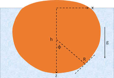
There are 3 interconnected equations governing the shape. They depend on b, h, σ, Δρ and on g, gravity. They relate to the angle φ which is 0 at the bottom of the drop and increases as you go upwards. The x-axis is horizontal and z is vertical. The radius of curvature at each point is R, with R=b at the lowest point. We then have:
- `(δx)/(δφ)=Rcosφ`
- `(δz)/(δφ)=Rsinφ`
- `1/R=(Δρg)/σ (h-z)+2/b-(sinφ)/x`
There is no analytical solution to this, so you just start at the bottom and step through small increments in φ. The numerics can explode when your settings don't match potential realities, so don't be alarmed by strange results.
Getting a good image
The technique for going from image to outline for you to fit is rudimentary - it depends on your threshold value. There are many more sophisticated image analysis techniques which might make shape extraction more accurate in the case of poorer-quality images. But experience shows that there's no substitute for a good original image. So pour your energies into a setup that is at the same time simple and reliable - and where the mm width of the image is a known constant. That's a lot of work, but it will pay off in terms of ease of measurement across multiple samples.
What happens at the surface?
Getting a good image of the basic shape is hard. At the interface between air and liquid, optical and physical effects combine to make it hard to have a meaningful combination of image and fit, so focus on the main shape (fit h and b as a priority) without worrying too much about a perfect fit at the top of the drop. Delightful concepts such as Neumann's Triangle might give you some small theoretical improvements at the expense of much extra work. So keep it simple.
Beyond the floating drop method
Young-Laplace applies to pendant drops from syringes and to bubbles in liquids. As long as you can define where the interesting stuff starts, so you can define h, the analysis should work just fine. However, sliders that cover the likely range of the floating drop method are ill-suited to gas bubbles. Maybe a separate Bubble-Young-Laplace will be needed.
1Masashi Nakamoto, Toshihiro Tanaka, Takaiku Yamamoto, Measurement of interfacial tension between oil and an aqueous solution via a floating drop method, Colloids and Surfaces A 529 (2017) 985–989
2Masashi Nakamoto, Yuko Kasai, Toshihiro Tanaka, Takaiku Yamamoto, Measurement of liquid/liquid interfacial tension with water on liquid paraffin by the floating drop method, Colloids and Surfaces A 603 (2020) 125250